An Anomaly-based alert in SigNoz allows you to define conditions based on metric data and trigger alerts when the metric data deviates from the expected behavior. Here's a breakdown of the various sections and options available when configuring an Anomaly-based alert:
Step 1: Define the Metric
In this step, you use the Metrics Query Builder to choose the metric to monitor. The following fields that are available in Metrics Query Builder includes:
Metric: A field to select the specific metric you want to monitor (e.g., CPU usage, memory utilization).
Time aggregation: A field to select the time aggregation function to use for the metric. Learn more about time aggregation
WHERE: A filter field to define specific conditions for the metric. You can apply logical operators like "IN," "NOT IN".
Space aggregation: A field to select the space aggregation function to use for the metric. Learn more about space aggregation
Legend Format: An optional field to customize the legend's format in the visual representation of the alert.
Having: Apply conditions to filter the results further based on aggregate value.
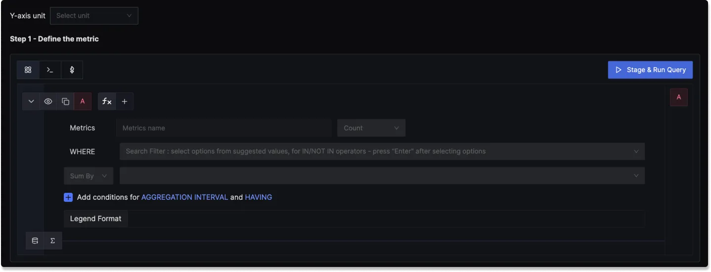
To know more about the functionalities of the Query Builder, checkout the documentation.
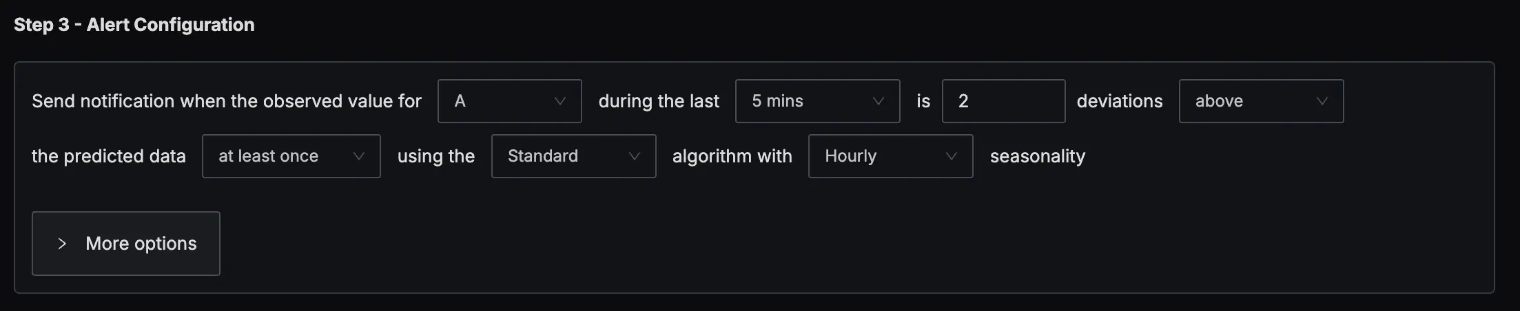
Step 2: Define Alert Conditions
In this step, you define the specific conditions that trigger the alert and the notification frequency. The following fields are available:
Evaluation window: Specify the rolling time window for the condition evaluation. The following look back options are available:
- Last 5 minutes
- Last 10 minutes
- Last 15 minutes
- Last 1 hour
- Last 4 hours
- Last 1 day
Z-score threshold: Specify the Z-score threshold for the alert condition.
Condition: Specify when the metric should trigger the notification
- Above threshold
- Below threshold
- Above or below threshold
Occurrence: Specify how condition should be evaluated
- At least once
- Every time
Algorithm: Specify the algorithm to use for the anomaly detection. The following algorithms are available:
- Standard
Seasonality: Specify the seasonality for the anomaly detection. The following seasonality options are available:
- Hourly
- Daily
- Weekly
More Options :
Run alert every [X mins]: This option determines the frequency at which the alert is evaluated.
Send a notification if data is missing for [X] mins: A field to specify if a notification should be sent when data is missing for a certain period.
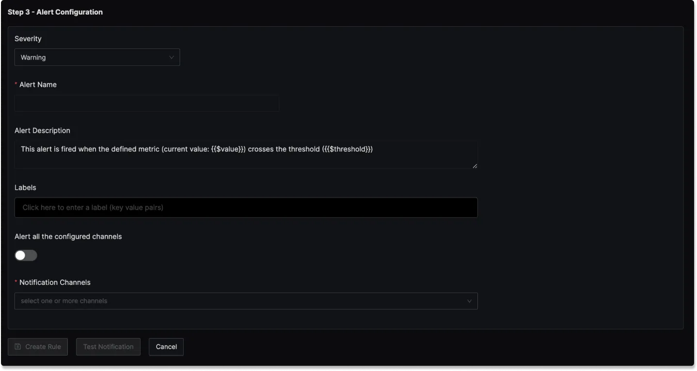
Step 3: Alert Configuration
In this step, you set the alert's metadata, including severity, name, and description:
Severity
Set the severity level for the alert (e.g., "Warning" or "Critical").
Alert Name
A field to name the alert for easy identification.
Alert Description
Add a detailed description for the alert, explaining its purpose and trigger conditions.
You can incorporate result attributes in the alert descriptions to make the alerts more informative:
Syntax: Use $<attribute-name> to insert attribute values. Attribute values can be any attribute used in group by.
Example: If you have a query that has the attribute service.name in the group by clause then to use it in the alert description, you will use $service.name.
Slack alert format
Using advanced slack formatting is supported if you are using Slack as a notification channel.
Labels
A field to add static labels or tags for categorization. Labels should be added in key value pairs. First enter key (avoid space in key) and set value.
Notification channels
A field to choose the notification channels from those configured in the Alert Channel settings.
Test Notification
A button to test the alert to ensure that it works as expected.
How It Works
The anomaly detection system uses a seasonal decomposition approach to identify unusual patterns in time series data. It learns from historical patterns and compares current values against predictions based on:
- Recent trends (immediate past behavior)
- Seasonal patterns (cyclical behavior)
- Historical growth trends (long-term changes)
Key Components
- Seasonality Types: Hourly, Daily, Weekly
- Evaluation Window: Configurable (we'll use 5 minutes in examples)
- Detection Method: Z-score based anomaly scoring
Core Algorithm
Formula
prediction = moving_avg(past_period) + avg(current_season) - mean(past_seasons)
             \____________________/   \________________/   \________________/
                      |                        |                    |
              Recent baseline         Seasonal growth      Historical average
Anomaly Score Calculation
anomaly_score = |actual_value - predicted_value| / stddev(current_season)
Detection Logic
if anomaly_score > z_score_threshold:
    Trigger
Hourly Seasonality
Time Window Breakdown
For evaluation at 3:05 PM (15:05):
| Window | Time Range | Purpose |
|---|---|---|
| Current Period | 15:00-15:05 today | Values being evaluated |
| Past Period | 13:55-14:00 today | Baseline from 1 hour ago |
| Current Season | 14:05-15:05 today | Last hour's trend |
| Past Season 1 | 13:05-14:05 today | 1-2 hours ago trend |
| Past Season 2 | 12:05-13:05 today | 2-3 hours ago trend |
| Past Season 3 | 11:05-12:05 today | 3-4 hours ago trend |
Example: E-commerce Checkout Service Latency
Data Pattern
# Evaluating at 3:05 PM for window 3:00-3:05 PM
# Normal pattern: spike at :00 due to promo emails, gradual decrease

Current Period (15:00-15:05):
  15:00: 250ms  # small spike from promo email traffic
  15:01: 220ms  # small but still elevated
  15:02: 180ms  # Normalizing
  15:03: 150ms  # Normal
  15:04: 145ms  # Normal
  15:05: 380ms  # Example of our interest!

Past Period (13:55-14:00):
  13:55: 140ms  # End of normal period
  13:56: 142ms
  13:57: 145ms
  13:58: 180ms  # Pre-spike buildup
  13:59: 210ms  # Pre-spike buildup
  14:00: 245ms  # Start of hourly spike

Historical Patterns:
  Current Season avg (14:05-15:05): 175ms
  Past Season 1 avg (13:05-14:05): 172ms
  Past Season 2 avg (12:05-13:05): 170ms
  Past Season 3 avg (11:05-12:05): 168ms

Standard Deviation: 35ms - entire season
Standard Deviation For Hourly Seasonality Example
The Current Season window is 14:05-15:05 (last hour). The system would have data points for this entire hour.
Current Season Data (14:05-15:05) - Full Hour:
  14:05: 145ms
  14:06: 148ms
  14:07: 152ms
  ...
  14:58: 165ms
  14:59: 195ms
  15:00: 250ms
  15:01: 220ms
  15:02: 180ms
  15:03: 150ms
  15:04: 145ms
  15:05: 380ms
Standard Deviation Formula
1. Calculate mean = Sum(values) / n
2. Calculate variance = Sum(value - mean)^2 / n
3. Standard deviation = sqrt(variance)
Detailed Calculation Example
Let's say we have 60 data points (one per minute) in the Current Season with this distribution:
Data Distribution:
- Normal range (140-160ms): 45 points
- Moderate spikes (180-220ms): 10 points
- High spikes (240-260ms): 5 points

Sample calculation with simplified data:
Values: [145, 148, 152, ..., 250, 220, 180, 150, 145]
Mean: 175ms

Variance calculation:
- (145-175)^2 = 900
- (148-175)^2 = 729
- (152-175)^2 = 529
- ...
- (250-175)^2 = 5625
- (220-175)^2 = 2025

Sum of squared differences: ~73,500
Variance (σ²): 73,500 / 60 = 1,225
Standard Deviation (σ): √1,225 = 35ms
Calculated from Current Season
The standard deviation is computed from the entire seasonal period, not just the evaluation window:
- Hourly: Last hour of data
- Daily: Last 24 hours of data
- Weekly: Last 7 days of data
Calculation for 15:05 spike
- Moving avg of past period: (140+142+145+180+210+245)/6 = 177ms
- Current season average: 175ms
- Historical mean: (172+170+168)/3 = 170ms
- Prediction: 177 + 175 - 170 = 182ms
- Actual value: 380ms
- Anomaly Score: |380 - 182| / 35 = 5.66
Result: ✅ Alert triggered (5.66 > 3.0 threshold)
Daily Seasonality
Time Window Breakdown
For evaluation on Tuesday 2:05 PM:
| Window | Time Range | Purpose |
|---|---|---|
| Current Period | Tue 14:00-14:05 | Values being evaluated |
| Past Period | Mon 13:55-14:00 | Same time yesterday |
| Current Season | Mon 14:05 - Tue 14:05 | Last 24 hours |
| Past Season 1 | Sun 14:05 - Mon 14:05 | 24-48 hours ago |
| Past Season 2 | Sat 14:05 - Sun 14:05 | 48-72 hours ago |
| Past Season 3 | Fri 14:05 - Sat 14:05 | 72-96 hours ago |
Example: Payment Gateway Transaction Volume
Context
A payment gateway with strong daily patterns:
- Business hours: 9 AM - 6 PM peak
- Lunch dip: 12 PM - 1 PM
- After-hours: minimal activity
- Weekend: 40% lower than weekdays
Data Pattern
# Evaluating Tuesday 2:05 PM for window 2:00-2:05 PM
# Expected: Post-lunch recovery period

Current Period (Tue 14:00-14:05):
  14:00: 8,500 txn/min   # Lunch recovery starting
  14:01: 9,200 txn/min   # Ramping up
  14:02: 9,800 txn/min   # Normal afternoon
  14:03: 10,100 txn/min  # Normal afternoon
  14:04: 9,900 txn/min   # Normal afternoon
  14:05: 4,200 txn/min   # Drop of interest!

Past Period (Mon 13:55-14:00):
  13:55: 7,800 txn/min   # End of lunch period
  13:56: 8,100 txn/min
  13:57: 8,400 txn/min
  13:58: 8,700 txn/min
  13:59: 9,000 txn/min
  14:00: 9,300 txn/min   # Recovery complete

Daily Patterns:
  Current Season avg (last 24h): 6,200 txn/min
  Past Season 1 avg (Mon): 6,100 txn/min
  Past Season 2 avg (Sun): 3,800 txn/min  # Weekend
  Past Season 3 avg (Sat): 3,600 txn/min  # Weekend

Standard Deviation: 2,500 txn/min
Calculation for 14:05 drop
- Moving avg of past period: ~8,550 txn/min
- Current season average: 6,200 txn/min
- Historical mean: (6,100+3,800+3,600)/3 = 4,500 txn/min
- Prediction: 8,550 + 6,200 - 4,500 = 10,250 txn/min
- Actual value: 4,200 txn/min
- Anomaly Score: |4,200 - 10,250| / 2,500 = 2.42
Result
Result: ❌ No alert (2.42 < 3.0 threshold)
While this is a significant drop, it doesn't exceed the threshold due to high variance from weekend data. You might want to use weekly seasonality for this metric to avoid weekend influence.
Weekly Seasonality
Time Window Breakdown
For evaluation on Week 4, Wednesday 10:05 AM:
| Window | Time Range | Purpose |
|---|---|---|
| Current Period | W4 Wed 10:00-10:05 | Values being evaluated |
| Past Period | W3 Wed 09:55-10:00 | Same time last week |
| Current Season | W3 Wed 10:05 - W4 Wed 10:05 | Last 7 days |
| Past Season 1 | W2 Wed 10:05 - W3 Wed 10:05 | 7-14 days ago |
| Past Season 2 | W1 Wed 10:05 - W2 Wed 10:05 | 14-21 days ago |
| Past Season 3 | W0 Wed 10:05 - W1 Wed 10:05 | 21-28 days ago |
Example: SaaS Application User Sessions
Data Pattern
# Evaluating Week 4, Wednesday 10:05 AM for window 10:00-10:05 AM
# Expected: Mid-week team sync spike around 10 AM

Current Period (W4 Wed 10:00-10:05):
  10:00: 12,000 sessions  # Start of sync meetings
  10:01: 14,500 sessions  # Spike building
  10:02: 16,200 sessions  # Peak sync time
  10:03: 15,800 sessions  # Still elevated
  10:04: 14,200 sessions  # Normalizing
  10:05: 13,500 sessions  # Normal

Past Period (W3 Wed 09:55-10:00):
  09:55: 10,500 sessions  # Pre-meeting normal
  09:56: 10,800 sessions
  09:57: 11,200 sessions  # People joining early
  09:58: 11,800 sessions
  09:59: 12,500 sessions  # Meeting prep
  10:00: 13,800 sessions  # Meetings starting

Weekly Patterns:
  Current Season avg (last 7 days): 8,500 sessions
  Past Season 1 avg (W2-W3): 8,200 sessions
  Past Season 2 avg (W1-W2): 8,000 sessions
  Past Season 3 avg (W0-W1): 7,800 sessions

Standard Deviation: 3,000 sessions
Normal Behavior Validation
For the 10:03 data point (15,800 sessions):
- Moving avg of past period: ~11,600 sessions
- Current season average: 8,500 sessions
- Historical mean: (8,200+8,000+7,800)/3 = 8,000 sessions
- Prediction: 11,600 + 8,500 - 8,000 = 12,100 sessions
- Actual value: 15,800 sessions
- Anomaly Score: |15,800 - 12,100| / 3,000 = 1.23
Result: (1.23 < 3.0) - This is an expected Wednesday spike
Z-Score Threshold Tuning
# Conservative (fewer alerts)
z_score_threshold: 4.0

# Balanced (default)
z_score_threshold: 3.0

# Sensitive (more alerts)
z_score_threshold: 2.5

# Very sensitive
z_score_threshold: 2.0
